In probability theory and statistics, the binomial distribution is the discrete probability distribution of the number of successes in a sequence of
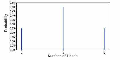
Binomial Probability Distribution
This is a graphic representation of a binomial probability distribution.
The binomial distribution is frequently used to model the number of successes in a sample of size
In general, if the random variable
For
Is the binomial coefficient (hence the name of the distribution) "n choose k," also denoted
One straightforward way to simulate a binomial random variable
Figures from the Example
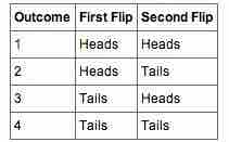
Table 1
These are the four possible outcomes from flipping a coin twice.
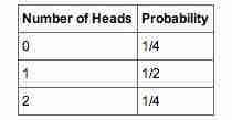
Table 2
These are the probabilities of the 2 coin flips.